Detecting Marine Winds from Space: An Introduction to Scatterometry and the Current Operational Scatterometers

Introduction

Weather analysis and forecasting over the open ocean remains a significant challenge given the relative lack of in-situ observed data as compared to terrestrial areas. While ship observations and buoys go a long way toward filling these gaps, there still exist areas of data void. Thus, forecasters must rely on satellite remote sensing techniques to fill in the large data gaps for these areas. The traditional application of satellite data has been weather surveillance for locating weather features and estimating their intensity based on cloud temperatures and patterns. This application, however, has some limitations since it provides little information on variables such as surface winds. Thus, estimating surface wind can be particularly problematic, especially if there are no nearby ship observations. More recently, a wealth of advanced satellite technology and instrumentation has been introduced, which now allows the estimation of surface and near-surface winds from space. One of the most applicable developments for the marine community is scatterometry, the only satellite-borne technology capable of estimating wind speed and direction with nearly global daily coverage. This paper provides a brief introduction into scatterometry, its application to the marine community, and a description of a new scatterometer instrument to begin operations during fall of 2003.

Scatterometry

Scatterometers are satellite-borne microwave radar instruments, which send out a series of specific signals or pulses and then measure how much of that signal or energy is returned. Microwaves have sufficiently high frequency to penetrate clouds, thus overcoming limitations of the more traditional weather satellites (e.g. Geostationary Operational Environmental Satellites or GOES), which measure lower-frequency infrared and visible radiation. The amount of energy returned to the instrument, also known as backscatter, is primarily a function of reflection and scattering off the ocean surface. This backscattered energy varies according to the sea surface roughness caused by small (on the order of centimeters) wind generated waves also known as capillary waves. Rough seas reflect a stronger signal than calm and this difference in backscattered energy is used to estimate the wind speed. The backscattered energy is technically a measure of surface stress rather than the near-surface wind, which means it must be converted to wind speed using empirical relationships (Atlas et al. 2001). The wind speed is also corrected for stability and adjusted to a standard height. Thus, wind measurements from scatterometers are indirect estimates, not observations, and reflect the wind speed at 10 meters under neutral stability (Atlas et al 2001). While the amount of backscatter determines the wind speed, the orientation of the backscattered energy with respect to propagation of the original pulse determines the wind direction. Scatterometers measure the amount of backscattered energy from multiple directions or different angles depending on their scanning geometry. This provides up to four different possible solutions for the wind direction. The most likely wind direction is determined by identifying the best fit between the wind direction and observed backscatter from the different angles. Typically, the best fit corresponds to the true direction while the next best fit corresponds to the opposite direction.

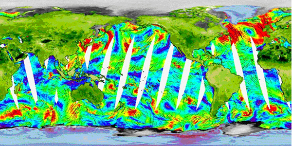
Scatterometer instruments are typically deployed on sun-synchronous near-polar-orbiting satellites that orbit the earth in a fashion such that they pass over the equator at approximately the same local times each day. These satellites orbit at an altitude of approximately 800 km (~ 500 statute miles) and are commonly known as Polar Orbiting Environmental Satellites (POES). This orbit and lower altitude differs from the more commonly known GOES satellites, which orbit above the equator at an elevation of 22,240 miles. GOES satellites orbit above the Earth at a speed which matches the Earth’s rotation, thus allowing them to hover or remain stationary over one position above the earth. Conversely, POES satellites complete fourteen daily near polar orbits each taking approximately 100 minutes to complete. This orbit allows roughly two passes over any geographical location per day. Modern scatterometers deployed on POES can thus provide nearly global daily coverage via a series of 1800 km wide swaths (Figure 1), as opposed to the GOES which has more limited overall coverage. Also, the POES lower earth orbit improves resolution, allowing more detailed monitoring of the ocean surface. Another difference between GOES and scatterometer instruments is that GOES sensors do not send out a signal but simply measure radiation emitted from the earth. For this reason, scatterometers are known as active sensors while sensors on the GOES are known as passive. Additionally, because scatterometers employ a microwave signal which can penetrate clouds, they can sample the earth’s surface under most weather conditions day and night. Conversely, GOES weather satellites are unable to see through cloud cover, thus limiting their ability to provide information of surface conditions during many weather situations.

Figure 1. First images from the new SeaWinds scatterometer on the Midori 2 satellite taken during January 28-29, 2003. The image shows the typical daily coverage (~ 93% of ocean surface) that can be achieved with modern scatterometers. White regions indicate unmeasured areas between the satellite swaths (viewing area).

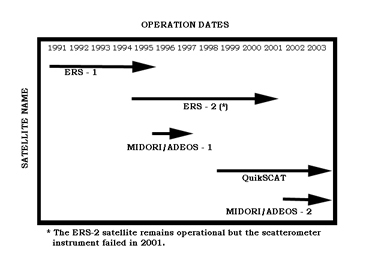Figure 2. Schematic illustration of past, present, and future scatterometer instruments.

Scatterometers Past and Present

The history of scatterometry dates back to World War II when radar observations over oceans contained clutter from signal returns off unknown sources. During the 1960s, this clutter was found to be due to the effects of wind. This led to the first tests of space based scatterometry during the Skylab missions of 1973 and 1974. These relatively short missions were followed by the deployment of the SeaSat-A Satellite Scatterometer (SASS). The SASS was a Ku band (microwave frequencies near 14 GHz) radar designed specifically for monitoring the ocean surface. It had antennas equipped on both sides of the satellite, which allowed for two simultaneous observational swaths approximately 500-km wide separated by a data free region called the nadir gap. The SASS mission operated from June through October of 1978 and demonstrated that accurate winds could be measured from space. The European Remote Sensing (ERS) satellites (Figure 2) later followed the SASS and marked the beginning of nearly continuous scatterometer coverage. The ERS satellites were equipped with a C band (~ 5 GHz) scatterometer with 25 km resolution. These scatterometers utilized three antennae that generated radar beams looking 45 degrees forward, sideways, and backward with respect to the satellite's flight direction.

The multiple beams allowed three different viewing angles of any particular point with different incidence angles and covered a 500 km-wide swath. The first ERS satellite (ERS-1) operated from 1991-1995 with the successor, ERS-2, becoming operational in 1995. While the ERS-2 satellite remains operational, the scatterometer failed in 2001. However, the radar altimeter equipped on the ERS-2 continues to provide sea height measurements. In 1996, the National Aeronautics and Space Administration (NASA) began a joint mission with the National Space Development Agency of Japan to maintain continuous scatterometer missions beyond ERS satellites. The first scatterometer via this joint effort was the NASA scatterometer (NSCAT) aboard the Advanced Earth Observing Satellite (ADEOS). The NSCAT was similar to SASS in that it employed antennas on each side of the satellite, allowing two simultaneous swaths but with slightly improved swath widths (~600-km). The Ku band NSCAT instrument operated with 50 km resolution and collected data for 9 months prior to prematurely losing power in 1997. NASA’s solution to the failed NSCAT was the QuikSCAT mission (for Quick Scatterometer), which was launched in 1999. To date, the QuikSCAT satellite remains in operation, far outlasting its 2-3 year mission life expectancy. The QuikSCAT mission includes a more advanced scatterometer instrument (called SeaWinds) that utilizes a conical scanning technique. This novel technique employs rotating dish antennae that eliminates the nadir gap and increases the swath width to approximately 1,800 km.

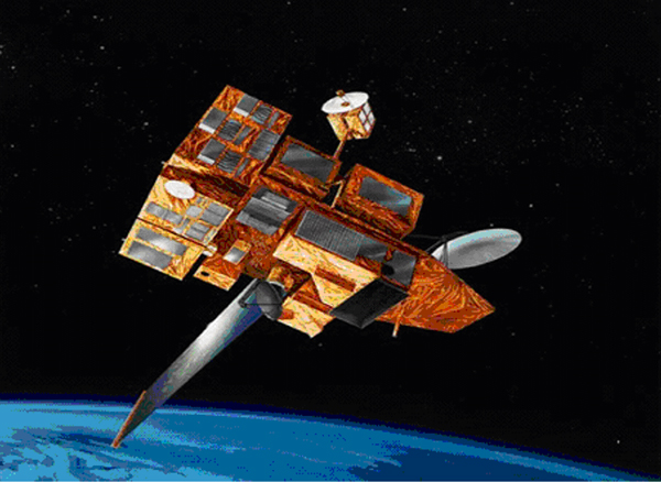Figure 3. SeaWinds scatterometer on the ADEOS-II/Midori 2.

The improved sampling size allows approximately 90% of the earth’s ocean surface to be sampled on a daily basis as opposed to two days by NSCAT and four days by the ERS instruments. The new scatterometer also has much improved horizontal resolution (25 km) over the 50 km NSCAT. Wind estimates taken by QuikSCAT are currently available to forecasters within about three hours of the observation time. Wind estimates are accurate within two meters/sec for speed and 20 degrees for direction in rain-free areas. The newest scatterometer instrument (commonly known as SeaWinds) was launched in December of 2002 onboard the ADEOS-2 satellite, later named Midori 2. SeaWinds on Midori 2 (Figure 3) is very similar to the SeaWinds on QuikSCAT and was first activated in January 2003. A six-month calibration/validation phase began in April, and regular operations are currently scheduled to begin this October. SeaWinds on Midori 2 will initially complement and eventually replace the existing QuikSCAT scatterometer. It is expected to last three to five years (Figure 2).

In addition to the SeaWinds scatterometer, the Midori 2 satellite is also equipped with an Advanced Microwave Scanning Radiometer (AMSR). The AMSR instrument detects microwave emissions from the Earth's surface and atmosphere and is able to measure various parameters such as precipitation. The ability to measure precipitation will allow for a more explicit detection of rain which can only be inferred from the current QuikSCAT instrument. This should improve the quality control of wind retrievals within and near areas of heavy rain, a major difficulty with the current QuikSCAT. This is discussed further in the limitations section below. An example of estimated surface marine winds from SeaWinds on Midori 2 is shown in Figure 1.

Marine Forecasting Application

There are many marine applications of scatterometer data including improved surface weather and sea state analyses, warnings, and forecasts. Scatterometers provide increased data availability over the oceans and fill in gaps between ship observations. The increased data aids in locating weather features such as fronts, troughs, high and low pressure centers, and surface circulations associated with developing tropical cyclones (TC).

These features can have a large impact on both the current and forecast wind field and sea state. Scatterometer data has also greatly improved the determination of the TC wind radii, which has far reaching implications for both marine interest as well as pre-landfall emergency preparations. Atlas et al. (2001) provide a more comprehensive discussion of the impacts of scatterometer data on operational forecasts. It should be noted that scatterometer data is not a replacement for ship observations. In fact, these two sources of marine observations can complement each other. For example, Rhome (2003) showed an example where a ship observation concurrent with QuikSCAT wind estimates helped validate storm force winds within the Gulf of Tehuantepec. In situations where both ship and scatterometer data are available, there is much more confidence in the issuance of warnings. Cobb et al. (2003) further showed the operational impact of QuikSCAT data for validating marine warnings.

One of the less commonly known applications of scatterometer data is improved initialization and evaluation of numerical weather prediction (NWP) models. Atlas et al. (2001) found that the ability of NWP to use scatterometer data has improved substantially. This has far reaching implications since accurate initialization of NWP models can be directly related to improved forecasts. Without accurate initial conditions, a model’s ability to provide accurate forecasts is severely limited. Imagine having very precise directions somewhere without knowing where to start. In effect, those directions are virtually useless. Meteorologists commonly use the phrase “garbage in equals garbage out” to convey that a numerical model with inaccurate initial conditions will produce an inaccurate forecast. For example, Atlas et al. (2001) showed an example from two powerful storms that affected France during December 1999. Control runs of NWP models without QuikSCAT data were unable to detect these features, leaving little warning time. However, similar NWP simulations with the QuikSCAT data included provided more evidence of the developing systems.

In addition to aiding the initialization of NWP models, scatterometer data also allows forecasters to evaluate the accuracy of the initialization. For example, a feature of interest depicted in NWP output can be compared against the corresponding scatterometer data to determine if that feature is accurately positioned with the correct intensity (i.e., wind speed). This type of analysis is more applicable during situations where scatterometer data becomes available after the model’s initialization process. If the NWP model does not properly resolve the particular weather feature in question, then adjustments must be made to the forecast from that model, and/or another model must be utilized. A number of new marine applications of scatterometer data have recently been discovered, including detecting the extent of sea ice and ice concentration, iceberg tracking, and monitoring ice shelves. These new applications should significantly improve marine forecasts and warnings, thus continuing the scatterometer’s legacy as the mariner’s eyes in the sky.

Limitations

Despite its many applications, scatterometer data is subject to several limitations and ambiguities, many of which can affect the availability and accuracy of the wind estimates. First, since scatterometers are deployed on polar orbiting satellites, data is only available at any given location approximately twice per day. This means that data is not updated continuously (as is the case with GOES satellites). Also the data is often outdated since it is delayed (by 3 hours for the current QuikSCAT). The forecaster must make adjustments, especially for cases of rapidly evolving weather systems, to compensate for the data delay.

Additionally, gaps exist between the sampling swaths. These gaps are largest over the equator, smaller over the midlatitudes, and non-existent near the poles (Figure 1). This means that the satellite swath can completely miss a particular region or weather system, thus providing little or no wind information for that area. The problem is often compounded since the sub-orbital tracks (track in reference to the earth’s surface) do not exactly repeat on a daily basis. The satellite swaths progress from east to west, even though the local solar time of each satellite's passage is essentially unchanged for any latitude.

Essentially, this means that the satellite swath can miss a westward-moving weather system during consecutive passes (often for many days) if the weather system moves at a speed similar to the satellite’s progression. In these cases, the scatterometer’s application is limited. Ambiguities in the retrieved wind direction are also a problem with scatterometer data. Scatterometers utilize measurements from multiple viewing angles in order to determine wind direction. Since these measurements provide up to four different solutions for direction, a best fit technique must be applied to determine the most likely direction among the possible solutions.

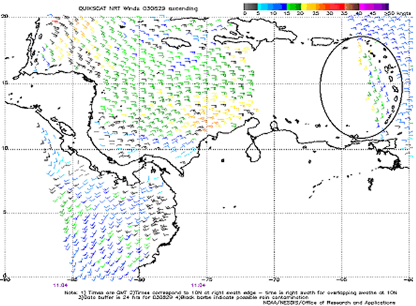
Figure 4. Example of typical swath edge contamination (shown in circled region) from the ascending pass of QuikSCAT during August 29, 2003. Note the southerly winds shown by QuikSCAT are 90 degrees off from the true easterly flow shown surrounding the encircled region."

Typically, the best fit corresponds to the true direction while the next best fit corresponds to the opposite direction. The process of determining the best fit can be complicated by noise within the data, especially at low wind speeds when the measured returned signal is weak. Also, determining the best fit is more difficult near the edges of the swath where there are relatively fewer observations due to the sampling process, and near the center of the swath where the ocean surface is viewed with a more limited set of incidence angles. Overall, the accuracy of wind directions near the swath edges, swath center, and within areas of weak flow is erroneous more often than strong winds in“sweet spots” of the swath on either side of the center (Figure 4).

Another limitation of scatterometers is that wind estimates are contaminated by heavy rain. This is caused by attenuation (reduction) of the signal as it travels to and from the ocean surface, increased scattering by the raindrops, and increased sea surface roughness caused by raindrop splashing on the ocean surface. For light wind conditions, heavy rain causes an overestimate of the wind speed, due to increased backscatter from the raindrops and increased roughness caused by splashing on the ocean surface. Conversely, rain contamination has a lesser effect on wind speed estimates in stronger wind situations since, the increased sea surface roughness caused by the wind will dominate over the rain effect. There are no sensors on the QuikSCAT satellite that can directly measure rain. Thus, identifying rain-contaminated retrievals is problematic. However, the post-processing of the QuikSCAT data includes a “rain flag” which alerts forecasters that certain wind estimates may be contaminated based on characteristics of the wind estimates that suggests that rain may be present.

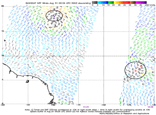
Figure 5. Examples of rain contaminates shown by black barbs within the encircled regions. The system near 500W is Hurricane Fabian and the system further east is an ITCZ disturbance. Both systems had deep convection over the areas highlighted.

These winds are often highly scrutinized by the forecaster or omitted altogether. Rain contamination can be a severe limitation especially for weather systems that cause deep convection such as tropical cyclones. An example from Hurricane Fabian (2003) is shown in Figure 5.

Rain flagging ability should be improved with the new SeaWinds scatterometer on Midori 2 since that satellite is also equipped with the AMSR instrument which can more directly measure precipitation. The above limitations of scatterometers can significantly affect the accuracy of the data and may present misleading information. In some cases, extensive experience and analysis is required to properly interpret that data and to compensate for untimely data. For this reason, mariners should use caution when making crucial decisions based solely on scatterometer information. The National Weather Service’s high seas and offshore forecasts incorporate forecaster interpretation of scatterometer data and other remotely sensed information as well as ship observations.

Acknowledgments

The author wishes to acknowledge the thoughtful comments by Dr. Richard Knabb, Dr. Chris Hennon, Christopher Burr, Robbie Berg, and Hugh Cobb which greatly aided in the composition of this paper. This article makes use of information presented on the Jet Propulsion Laboratory webpage (www.jpl.nasa.gov). For more information on the new SeaWinds scatterometer on Midori 2, see http://winds.jpl.nasa.gov/news/index.html.

Biography

Jamie Rhome has worked as a meteorologist/forecaster for the Tropical Analysis and Forecast Branch of the Tropical Prediction Center since September 1999. He received his B.S. and M.S degrees in Meteorology from North Carolina State University. Previous work experience includes the United States Environmental Protection Agency and the State Climate Office of North Carolina at North Carolina State University.

References

Atlas, R., R.N. Hoffman, S.M. Leidner, J. Sienkiewicz, T.-W.Yu, S.C. Bloom, E. Brin, J. Ardizzone, J. Terry, D. Bungato, and J.C. Jusem, 2001: The effects of marine winds from scatterometer data on weather analysis and forecasting. Bulletin of the American Meteorological Society, Vol 82, No. 9, 1965-1990.

Cobb, H.D., D.P. Brown, and R. Molleda, 2003: The use of QuikSCAT imagery in the diagnosis and detection of Gulf of Tehuantepec wind events 1999-2002. Preprints 12th Conference on Satellite Meteorology and Oceanography. Long Beach, CA 9-13 Feb. 2003. PP 410.

Rhome, J.R., 2003: Application and use of volunteer observing ship (VOS) data at the Tropical Prediction Center/National Hurricane Center. Mariners Weather Log. Spring/Summer, 2003.

Page last modified: